### load libraries ###
library(tidyverse)
library(here)
library(janitor)
library(showtext)
library(ggsankey)
library(patchwork)
### read in data ###
# counts
counts <- read_csv(here("data", "Count_All_DataRaw.csv")) %>%
clean_names() %>%
remove_empty(c("rows", "cols"))
# spawning
spawn <- read_csv(here("data", "Spawning_All_DataRaw.csv")) %>%
clean_names() %>%
remove_empty(c("rows", "cols"))
#pedigree
pedigree <- read_csv(here("data", "White_Abalone_Pedigree_Data_Metadata(Pedigree).csv")) %>%
clean_names() %>%
remove_empty(c("rows", "cols"))
# transfer
transfer <- read_csv(here("data", "Transfer_All_DataRaw.csv")) %>%
clean_names() %>%
remove_empty(c("rows", "cols"))
### wrangle data ###
# counts
counts <- counts %>%
mutate(pop_id = case_when(
pop_id == "16-03-02-Acjachemen,\n16-03-12-Tongva,\n16-03-02-Miwok,\n16-03-02-Pomo" ~ "16-03-02-NativeTribes",
pop_id == "17-03-01-Merida, 17-03-01-Tiana" ~ "17-03-01-Tiana/Merida",
pop_id == "17-03-01-Tiana, 17-03-01-Merida" ~ "17-03-01-Tiana/Merida",
pop_id == "16-03-02-Acjachemen, 16-03-02-Tongua, 16-03-02-Miwok, 16-03-02-Pomo" ~ "16-03-02-NativeTribes",
pop_id == "22-05-10-Bubbles, 22-05-10-Blossom" ~ "22-05-10-Bubbles/Blossom",
pop_id == "19-04-16-Spongebob, 19-04-16-Patrick" ~ "19-04-16-Spongebob/Patrick",
pop_id == "19-04-16-Squidward, 18-04-19-Ursula" ~ "19-04-16-Squidward/Ursula",
pop_id == "21-04-21-Moderna,\n21-04-21-Pfizer,\n21-04-29-JandJ" ~ "21-04-21-Vaccines",
pop_id == "17-03-01-Tiana,\n17-03-01-Merida" ~ "17-03-01-Tiana/Merida",
pop_id == "16-03-02-Acjachemen, 16-03-02-Chumash, 16-03-02-Tongva, 16-03-02-Miwok, 16-03-02-Pomo" ~ "16-03-02-NativeTribes",
pop_id == "22-03-01-Mardi, 22-03-09-WALLE" ~ "22-03-01-Mardi/WALLE",
pop_id == "22-03-01-Mardi, 22-03-09-Walle" ~ "22-03-01-Mardi/WALLE",
pop_id == "17-03-01-Belle, 16-03-02-Acjachemen, 16-03-02-Tongva, 16-03-02-Miwok, 16-03-02-Pomo, 16-03-02-Chumash,19-04-16-Squidward, 18-04-19-Ursula, 19-04-16-Spongebob, 19-04-16-Patrick, 17-03-01-Tiana, 17-03-01-Merida, 20-03-10-Smaug" ~ "20-03-10-Mixed",
pop_id == "16-03-02-Acjachemen, 16-03-02-Tongva, 16-03-02-Miwok, 16-03-02-Pomo, 16-03-02-Chumash" ~ "16-03-02-NativeTribes",
pop_id == "17-03-01-Belle,16-03-02-Acjachemen, 16-03-02-Tongva, 16-03-02-Miwok, 16-03-02-Pomo, 16-03-02-Chumash" ~ "16-03-02-NativeTribes/Belle",
pop_id == "25-01-07-Hammerhead, 25-01-07-Nurse, 25-01-07-Epaulette" ~ "25-01-07-Sharks",
TRUE ~ pop_id
))
counts_clean <- counts %>%
filter(rack_type != "BST") %>%
mutate(year = year(date)) %>%
#counts_clean <- counts_clean %>%
filter(facility == "BML") %>%
group_by(date) %>%
summarise(count = sum(count, na.rm = TRUE)) %>%
ungroup() %>%
mutate(type = "counts")
# spawning
spawn <- spawn %>%
mutate(pop_id = case_when(
pop_id == "14-04-23-Beaker, 14-05-13-Fozzie" ~ "14-05-13-Fozzie/Beaker",
pop_id == "17-03-01-Tiana, 17-03-01-Merida" ~ "17-03-01-Tiana/Merida",
pop_id == "19-04-16-Squidward, 18-04-19-Ursula" ~ "19-04-16-Squidward/Ursula",
pop_id == "16-03-02-Acjachemen, 16-03-02-Tongva, 16-03-02-Miwok, 16-03-02-Pomo, 16-03-02-Chumash" ~ "16-03-02-NativeTribes",
pop_id == "19-04-16-Spongebob, 19-04-16-Patrick" ~ "19-04-16-Spongebob/Patrick",
pop_id == "14-04-30-Beaker,14-05-13-Fozzie" ~ "14-05-13-Fozzie/Beaker",
pop_id == "16-03-02-Acjachemen, 16-03-02-Tongva, 16-03-02-Miwok, 16-03-02-Pomo, 16-03-02-Chumash, 16-03-02-Kumeyaay, 16-03-02-Salinan" ~ "16-03-02-NativeTribes",
pop_id == "16-03-02-Acjachemen, 16-03-12-Tongva, 16-03-02-Miwok, 16-03-02-Pomo, 16-03-02-Chumash" ~ "16-03-02-NativeTribes",
pop_id == "17-03-01-Belle, 16-03-02-Acjachemen, 16-03-02-Tongva, 16-03-02-Miwok, 16-03-02-Pomo, 16-03-02-Chumash" ~ "16-03-02-NativeTribes/Belle",
pop_id == "19-04-16-Squidward/18-04-19-Ursula" ~ "19-04-16-Squidward/Ursula",
pop_id == "17-03-01-Tiana/17-03-01-Merida" ~ "17-03-01-Tiana/Merida",
pop_id == "16-03-02-Acjachemen/16-03-02-Tongva/16-03-02-Miwok/16-03-02-Pomo/16-03-02-Chumash" ~ "16-03-02-NativeTribes",
pop_id == "19-04-16-Spongebob/19-04-16-Patrick" ~ "19-04-16-Spongebob/Patrick",
pop_id == "07-05-19-Jeffrey" ~ "17-05-19-Jeffrey",
TRUE ~ pop_id
))
spawn_clean <- spawn %>%
# remove unknown popID since no date
filter(pop_id != "NA",
pop_id != "UNKNOWN") %>%
mutate(born = str_sub(pop_id, start = 1, end = 8), # pull out years from pop ID
born = as.Date(born, format = "%y-%m-%d"),
# fix date for swedish fish pop since only year
born = case_when(pop_id == "03-F1-SwedishChef" ~ as.Date("2003-01-01"),
TRUE ~ born),
# calculate age at spawn date
age = floor(time_length(interval(born, date), "years")),
egg_count = as.numeric(egg_count)) %>%
# add 5 years to wilds, since we do not know their age
mutate(age = case_when(pop_id == "04-12-05-Redwood" ~ age + 5,
pop_id == "17-01-31-Loblolly" ~ age + 5,
pop_id == "17-06-09-Sugar" ~ age + 5,
pop_id == "17-05-19-Jeffrey" ~ age + 5,
pop_id == "17-03-15-Ponderosa" ~ age + 5,
pop_id == "17-04-12-Torrey" ~ age + 5,
pop_id == "19-03-18-Ash" ~ age + 5,
pop_id == "17-11-13-Sequoia" ~ age + 5,
TRUE ~ age))
# transfer
transfer_clean <- transfer %>%
filter(life_stage == "settled") %>%
# transform any variable with outplant or growout into only 'outplant'
mutate(transport_purpose = case_when(
transport_purpose == "Outplant" ~ "outplant",
transport_purpose == "Outplant, Growout" ~ "outplant",
transport_purpose == "growout, outplant" ~ "outplant",
transport_purpose == "Growout" ~ "outplant",
transport_purpose == "grow-out" ~ "outplant",
transport_purpose == "growout" ~ "outplant",
TRUE ~ transport_purpose))
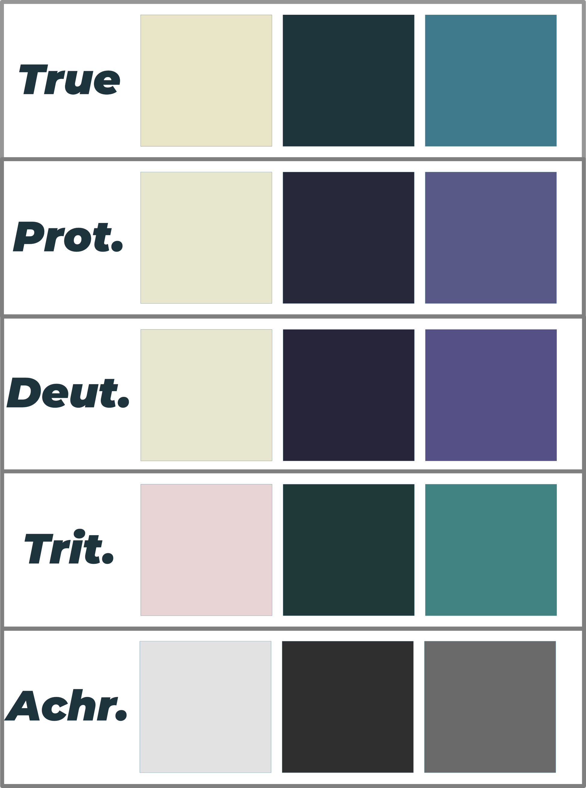
### initialize color theme ###
pal <- c("background" = "#E9E5C7",
"dark" = "#1F363D",
"light" = "#40798C",
"lightsteel" = "#CFDEE7")
### initialize fonts ###
font_add_google(name = "Zalando Sans Expanded", family = "zalando")
font_add_google(name = "Montserrat", family = "montserrat")
### Plot 1: heatmap ###
# wrangle data
spawn_clean <- spawn_clean %>%
mutate(sex = ifelse(!is.na(egg_count), "F", NA)) %>%
mutate(sex = ifelse(!is.na(time_initial_spawn) & is.na(egg_count), "M", sex))
spawn_female <- spawn_clean %>%
filter(!is.na(sex),
sex == "F") %>%
group_by(age, sex) %>%
summarise(egg_count = sum(egg_count)) %>%
ungroup() %>%
mutate(ratio = egg_count / max(egg_count))
spawn_male <- spawn_clean %>%
filter(!is.na(sex),
sex == "M") %>%
group_by(age, sex) %>%
summarise(n = n()) %>%
ungroup() %>%
mutate(ratio = n / max(n))
spawn_plot <- full_join(spawn_female, spawn_male)
# plot
showtext_auto(enable = TRUE)
annotation_heatmap1 <- glue::glue(
"No abalone have spawned
at these ages in captivity")
heatmap <- ggplot(spawn_plot, aes(x = age, y = sex, fill = ratio)) +
geom_tile() +
coord_fixed() +
annotate(geom = "text",
x = 16, y = 1.5,
label = annotation_heatmap1,
color = pal['dark'],
hjust = "center",
family = "montserrat") +
scale_fill_gradient(low = pal['steel'], high = pal["dark"]) +
theme_classic(base_size = 15) +
labs(title = "White abalone reproductive output by age and sex",
subtitle = "Peak spawning age is around 5 years old") +
theme(legend.direction = "horizontal",
legend.position = "bottom",
panel.background = element_rect(fill = pal['background']),
plot.background = element_rect(fill = pal['background']),
plot.title = ggtext::element_markdown(family = "zalando",
color = pal['dark']),
legend.box.background = element_blank()) +
guides(fill = guide_colorbar(title = "Reproductive\nOutput",
barwidth = 15, barheight = 1))
showtext_auto(enable = FALSE)
### Plot 2: histogram ###
# wrangle data
transfer_outplant <- transfer_clean %>%
filter(#transport_purpose == "outplant",
origin_facility == "BML") %>%
group_by(date) %>%
summarise(count = sum(as.numeric(numberofanimals), na.rm = TRUE)) %>%
ungroup() %>%
mutate(type = "transfer")
counts_outplant <- full_join(transfer_outplant, counts_clean) %>%
mutate(year = year(date)) %>%
group_by(year, type) %>%
summarise(count = round(sum(count))) %>%
ungroup() %>%
filter(year != 2025)
# plot
years <- c("2016", "2017", "2018", "2019", "2020", "2021", "2022", "2023", "2024")
breaks <- c(2016, 2017, 2018, 2019, 2020, 2021, 2022, 2023, 2024)
title <- glue::glue(
"Juvenile
<span style='color:#40798C;'>White Abalone</span>
and
<span style='color:#1F363D;'>outplanting</span>
counts"
)
annotation_histo1 <- glue::glue(
"COVID-19 Shutdown
decreased production")
annotation_histo2 <- glue::glue(
"Lagged effect from
COVID-19 Shutdown")
showtext_auto(enable = TRUE)
histogram <- ggplot(counts_outplant %>% filter(type == "counts"),
aes(x = year, y = count)) +
geom_col(width = .85, fill = pal["light"]) +
geom_smooth(data = counts_outplant %>% filter(type == "counts"),
se = FALSE, color = pal["light"]) +
geom_col(data = counts_outplant %>% filter(type == "transfer"),
aes(x = year, y = count),
fill = pal['dark'], width = .5) +
geom_smooth(data = counts_outplant %>% filter(type == "transfer"),
se = FALSE, color = pal['dark']) +
annotate(geom = "text",
x = 2020, y = 20000,
label = annotation_histo1,
color = pal['dark'],
hjust = "center",
family = "montserrat",
size = 8) +
annotate(geom = "text",
x = 2023.5, y = 10000,
label = annotation_histo2,
color = pal['dark'],
hjust = "center",
family = "montserrat",
size = 8) +
labs(title = title,
) +
theme(base_size = 10,
panel.background = element_rect(fill = pal['background']),
plot.background = element_rect(fill = pal['background']),
panel.grid.major = element_blank(),
panel.grid.minor = element_blank(),
plot.title = ggtext::element_markdown(family = "zalando",
color = "#040D10",
size = rel(3)),
axis.title.y = element_blank(),
axis.ticks.y = element_blank(),
axis.text.y = element_blank(),
axis.text.x = element_text(size = rel(2),
family = "montserrat"),
axis.title.x = element_text(size = rel(2.5),
family = "montserrat")) +
scale_x_continuous(breaks = breaks,
labels = years)
showtext_auto(enable = FALSE)
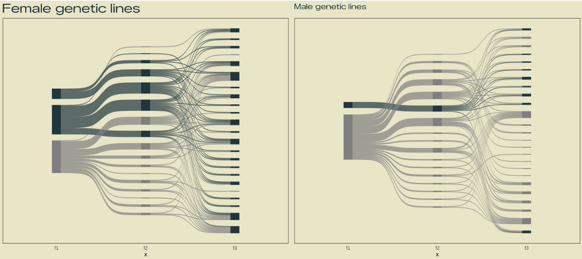
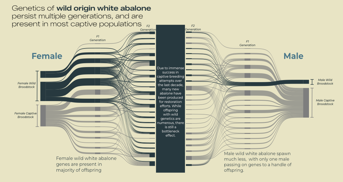
# Plot 3: Sankey ###
# wrangle data for female
pedigree_f <- pedigree %>%
filter(!is.na(mother_pop_id)) %>%
#filter(if_any(c(mother_pop_id), ~str_detect(., test))) %>%
select(pop_id, mother_pop_id) %>%
separate_longer_delim(mother_pop_id, delim = ", ") %>%
separate_longer_delim(mother_pop_id, delim = "/") %>%
separate_longer_delim(mother_pop_id, delim = ";") %>%
separate_longer_delim(mother_pop_id, delim = " OR ") %>%
mutate(mother_pop_id = case_when(
mother_pop_id == "01-04-23-Scooter (GRN_310)" ~ "01-04-23-Scooter",
mother_pop_id == "13-04-04-Rowlf (ORN_032)" ~ "13-04-04-Rowlf",
mother_pop_id == "Parental PopIDs possible: 16-03-02-Acjachemen" ~ "16-03-02-Acjachemen",
mother_pop_id == "SEE NOTES. N=6 females:\nN=2 18-04-09-Ursula (NYL_667" ~ "18-04-09-Ursula",
mother_pop_id == "\nN=1 19-04-16-Patrick (NYL_681)" ~ "19-04-16-Patrick",
mother_pop_id == "\nN=1 16-03-02-Acjachemen" ~ "16-03-02-Acjachemen",
mother_pop_id == "16-03-02-Chumash (LAV_063)" ~ "16-03-02-Chumash",
mother_pop_id == "01-04-23-Scooter (GRN_364)" ~ "01-04-23-Scooter",
mother_pop_id == "13-04-04-Rowlf (ORN_017)" ~ "13-04-04-Rowlf",
mother_pop_id == "\nN=1 19-04-16-Spongebob (NGN_624)" ~ "19-04-16-Spongebob",
mother_pop_id == "17-03-01-Tiana (LAV_006)" ~ "17-03-01-Tiana",
mother_pop_id == "\nN=1 17-03-01-Merida" ~ "17-03-01-Merida",
mother_pop_id == "20-03-10-Smaug\n" ~ "20-03-10-Smaug",
TRUE ~ mother_pop_id
)) %>%
filter(mother_pop_id != "NYL_677)",
mother_pop_id != "Unknown PopID BST Tank 5")
# pull out broodstock and join direct descendents
pedigree_f_brood <- tibble(unique(pedigree_f$mother_pop_id)) %>%
rename(mother_pop_id = "unique(pedigree_f$mother_pop_id)") %>%
left_join(pedigree_f) %>%
rename(f1 = mother_pop_id,
mother_pop_id = pop_id)
# pull out f1 generation popid's
pedigree_f_1 <- pedigree_f_brood %>%
filter(!f1 %in% mother_pop_id)
# pull out f2 generation popid's
pedigree_f_2 <- pedigree_f_brood %>%
filter(f1 %in% mother_pop_id) %>%
rename(mother_pop_id = f1,
f3 = mother_pop_id)
# join f1 and f2 generation to broodstock and make long for sankey
pedigree_f_long <- pedigree_f_1 %>%
left_join(pedigree_f_2) %>%
rename(f2 = mother_pop_id) %>%
filter(!is.na(f3)) %>%
make_long(f1, f2, f3)
# plot female
showtext_auto(enable = TRUE)
ped_female <- ggplot(pedigree_f_long, aes(x = x,
next_x = next_x,
node = node,
next_node = next_node,
fill = factor(node),
label = node)) +
geom_sankey(flow.alpha = 0.7,
show.legend = FALSE) +
scale_fill_manual(values = c('17-03-15-Ponderosa' = "#1F363D",
'17-01-31-Loblolly' ="#1F363D",
'17-03-01-Tiana' = "#1F363D",
"19-04-16-Plankton" = "#1F363D",
"19-04-16-Spongebob" = "#1F363D",
"19-04-16-Patrick" = "#1F363D",
"21-04-21-BioNTech" = "#1F363D",
"19-04-16-Squidward" = "#1F363D",
"20-03-10-Smaug" = "#1F363D",
"22-02-10-Ciri" = "#1F363D",
"22-05-10-Buttercup" = "#1F363D",
"24-02-13-Cormorant" = "#1F363D",
"23-02-08-Eevee" = "#1F363D",
"23-02-08-Polywag" = "#1F363D",
"23-04-05-Fiona" = "#1F363D",
"23-04-05-Farquaad" = "#1F363D",
"23-05-17-Funktopus" = "#1F363D",
"23-11-18-Artichoke" = "#1F363D",
"24-02-13-Goldfinch" = "#1F363D",
"24-02-13-Scrubjay" = "#1F363D",
"25-01-07-Nurse" = "#1F363D",
"25-03-11-Merry" = "#1F363D",
"25-03-11-Samwise" = "#1F363D",
"25-03-11-Rosie" = "#1F363D",
"25-05-15-Cauliflower" = "#1F363D",
"24-02-13-Peregrine" = "#1F363D",
"24-02-13-Seagull" = "#1F363D",
"25-01-07-Sevengill" = "#1F363D",
"25-01-07-Whale" = "#1F363D",
"25-03-11-Bilbo" = "#1F363D")) +
labs(title = "Female genetic lines") +
theme_minimal(base_size = 15) +
theme(panel.background = element_rect(fill = pal['background']),
plot.background = element_rect(fill = pal['background']),
axis.text.y = element_blank(),
panel.grid.major = element_blank(),
panel.grid.minor = element_blank(),
plot.title = ggtext::element_markdown(family = "zalando",
color = pal['dark']))
showtext_auto(enable = FALSE)
# wrangle data for male
pedigree_m <- pedigree %>%
filter(!is.na(father_pop_id)) %>%
select(pop_id, father_pop_id) %>%
separate_longer_delim(father_pop_id, delim = ", ") %>%
separate_longer_delim(father_pop_id, delim = "/") %>%
separate_longer_delim(father_pop_id, delim = ";") %>%
separate_longer_delim(father_pop_id, delim = " OR ") %>%
separate_longer_delim(father_pop_id, delim = ",") %>%
separate_longer_delim(father_pop_id, delim = "\n") %>%
mutate(father_pop_id = case_when(
father_pop_id == "Parental PopIDs possible: 16-03-02-Acjachemen" ~ "16-03-02-Acjachemen",
father_pop_id == "13-04-04-Rowlf and" ~ "13-04-04-Rowlf",
father_pop_id == "or 13-03-02-Janice" ~ "13-03-02-Janice",
father_pop_id == "17-03-01-Merida (WHT_159)" ~ "17-03-01-Merida",
father_pop_id == "17-03-01-Belle (WHT(TAN?)_222)" ~ "17-03-01-Belle",
father_pop_id == "Jabalone Expt: 18-04-19-Ursula (NYL_672)" ~ "18-04-19-Ursula",
father_pop_id == "18-04-19-Ursula (NYL_669)" ~ "18-04-19-Ursula",
father_pop_id == "17-03-01-Belle (NGN_151)" ~ "17-03-01-Belle",
father_pop_id == "01-04-23-Scooter (GRN_371" ~ "01-04-23-Scooter",
father_pop_id == "13-03-02-Janice (ORN_001)" ~ "13-03-02-Janice",
father_pop_id == "01-04-23-Scooter(GRN_305" ~ "01-04-23-Scooter",
father_pop_id == "\n17-03-01-Belle (n=1) " ~ "17-03-01-Belle",
father_pop_id == "16-03-02-Salinan (n=1)" ~ "16-03-02-Salinan",
father_pop_id == "17-03-01-Belle (n=1) " ~ "17-03-01-Belle",
TRUE ~ father_pop_id
)) %>%
filter(father_pop_id != "",
father_pop_id != "GRN_371)",
father_pop_id != "GRN_305)")
# pull out broodstock popid's
pedigree_m_brood <- tibble(unique(pedigree_m$father_pop_id)) %>%
rename(father_pop_id = "unique(pedigree_m$father_pop_id)") %>%
left_join(pedigree_m) %>%
rename(f1 = father_pop_id,
father_pop_id = pop_id)
# pull out f1 generation popid's
pedigree_m_1 <- pedigree_m_brood %>%
filter(!f1 %in% father_pop_id)
# pull out f2 generation popid's
pedigree_m_2 <- pedigree_m_brood %>%
filter(f1 %in% father_pop_id) %>%
rename(father_pop_id = f1,
f3 = father_pop_id)
# join f1 and f2 generation to broodstock and make long for sankey
pedigree_m_long <- pedigree_m_1 %>%
left_join(pedigree_m_2) %>%
rename(f2 = father_pop_id) %>%
filter(!is.na(f3)) %>%
make_long(f1, f2, f3)
# plot male
showtext_auto(enable = TRUE)
ped_male <- ggplot(pedigree_m_long, aes(x = x,
next_x = next_x,
node = node,
next_node = next_node,
fill = factor(node),
label = node)) +
geom_sankey(flow.alpha = 0.7,
show.legend = FALSE) +
scale_fill_manual(values = c('17-11-13-Sequoia' = "#1F363D",
"19-04-16-Patrick" = "#1F363D",
"23-11-18-Artichoke" = "#1F363D",
'24-02-13-Goldfinch' = "#1F363D",
"24-02-13-Osprey" = "#1F363D",
"24-02-13-Scrubjay" = "#1F363D",
"24-02-13-Seagull" = "#1F363D",
"24-04-23-Nemo" = "#1F363D",
"25-01-07-Epaulette" = "#1F363D",
"2025-01-07-Rocky" = "#1F363D",
"25-05-15-Cauliflower" = "#1F363D"
)) +
labs(title = "Male genetic lines") +
theme_minimal(base_size = 15) +
theme(axis.text.y = element_blank(),
panel.background = element_rect(fill = pal['background']),
plot.background = element_rect(fill = pal['background']),
panel.grid.major = element_blank(),
panel.grid.minor = element_blank(),
plot.title = ggtext::element_markdown(family = "zalando",
color = pal['dark']))
showtext_auto(enable = FALSE)
# join male and female plots together
sankey <- (ped_female | ped_male)
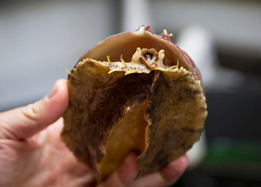 Image of the underside of a white abalone.